Faster Mandelbrot Set Rendering with BLA: Bivariate Linear Approximation

The latest and greatest (as of the time of writing, in May 2023) method for computing Mandelbrot set images is a form of bivariate linear approximation, which is referred to as BLA. Discussion of this method began in late 2021 on the fractalforums.org site (from the first post on page 3 of this thread). I made some failed attempts to implement BLA in 2022, but over the last few months I've finally got an experimental BLA working in my JavaScript Mandelbrot set viewer, Very Plotter.

In this post I'll show how to use BLA in the Very Plotter v0.10.0 release. Then, I'll give some background on the theory and implementation of BLA, and show the performance I'm seeing at some example locations.

Using BLA in Very Plotter

Before describing BLA itself, I'll show how to use it in Very Plotter, and what to expect.

As of Very Plotter v0.10.0, BLA should be considered an "experimental" feature. It works for many locations, but some locations have no acceleration provided by BLA and would be better viewed with plain perturbation theory or perturbation with series approximation.

To enable BLA in Very Plotter, open the controls menu (with the wrench icon) and expand the "algorithm options" pane. There, you'll find an "automatic with BLA" setting in the options dropdown list. Select that, and click the "Go" button.

With that "algorithm" active, BLA will be enabled once a sufficiently deep location is rendered (where the scale is greater than 1e25 pixels per unit).

When a BLA render starts, the following steps occur:

1. An on-screen minibrot nucleus is located
2. A reference orbit is calculated for a point in that nucleus
3. An $\epsilon$ (epsilon) value is found
4. BLAs are calculated using the $\epsilon$
5. Each pixel is computed using BLA, where iterations can be skipped, and using perturbation theory where individual iterations have no valid BLA

The first three steps above can take some time, during which the render window will show only status updates, and no actual rendered pixels. For very deep locations, those initial steps can take several minutes (or even hours, but for those locations you're much better off using a proper desktop Mandelbrot set viewer).

For some locations, the above step 1 currently fails. If a nucleus cannot be found, a periodic point cannot be found, and the middle of screen is used for the reference orbit point instead. This works fine for perturbation theory and for series approximation, but for my BLA implementation this slows things down considerably.

If, however, you are rendering a location with a found on-screen nucleus, you can use the R key to toggle on the mouse position display. You'll also see an "X" shape drawn on the found periodic point within a nucleus. If you draw a zoom box (hold alt/option and drag the mouse) that contains that point, steps 1 and 2 above can be skipped for the new zoomed-in location and rendering of the new location will start quickly. You can also re-use the reference orbit point by changing the scale or magnification in the "go to location by center and scale" pane in the controls menu.

Finding A Periodic Point

If we can find a periodic point on screen, then the reference orbit can be computed only for the period (since it repeats). Also, we will compute and merge fewer BLAs associated with that period-shortened reference orbit (more on that later). This significantly increases the overall speed with which we can find valid BLAs when computing each pixel (again, more on this later). So therefore, for performance reasons, it's worth taking the time to find an on-screen periodic point.

All points in the interior of the Mandelbrot set are periodic (by definition) so all we need to do is find a minibrot (or "mu-molecule") which luckily is a relatively straightforward, repeatable procedure:

1. Find the dominant period ("atom domain") of the window
2. Use the period in calculating Newton's method iterations to get progressively closer to the minibrot
3. If the minibrot is on-screen, we are done, otherwise, go back to step 1 to find a "deeper" higher-period minibrot

There are a few period-finding algorithms. One method involves iterating the points of a polygon (see "Finding the Period of a mu-Atom" on this page) but a faster method is the "ball arithmetic" method. I don't understand the math myself, but I was able to implement the method using the pseudocode from gerrit's post here. The "2nd order" algorithm ran too slowly for me, so I just use the "1st order" one. For the dx and dy parameters, I use the distance from the center of the screen to the edge of the screen, along the x and y axis respectively, which causes the algorithm to search within the largest possible circle that fits in the window being rendered. Step 3 above uses the doCont condition in the algorithm: continue iterating to find a deeper and higher period domain within the window.

Really helpful pseudocode for Newton's method was posted by claude here. To determine when Newton's method "starts to converge" I implemented an "approximately equals" method for my arbitrary precision numbers, which compares some number of most-significant digits.

Once we have a periodic point, we can compute only one period's worth of iterations for a reference orbit at that point.

Calculating the BLA Coefficients

Once we have our reference orbit, calculated with full precision, we can calculate a set of BLAs for it, where for each iteration $m$ in the reference orbit we can calculate coefficients $A_{\mathrm{l}}$ and $B_{\mathrm{l}}$ that allow us to skip ahead $l$ iterations.

Zhuoran provided an overview of the idea, with some nicely-formatted math, in this post. I ended up using their initial values and formulas for $A_0,B_0,A_1,B_1$ but not the generalized $A_l$ and $B_l$.

How many iterations do we skip? Recall that in perturbation theory, we can iterate our low-precision $\mathrm{\Delta }z$ with:

$${\mathrm{\Delta }z}_{\mathrm{n+1}}=2Z_n{\mathrm{\Delta }z}_n+{\mathrm{\Delta }z}_n^2+\mathrm{\Delta }c$$ $$\text{<small>where</small>}$$ $$Z_n=\text{<small>reference orbit at iteration </small>}n$$ $$z_n=\text{<small>pixel orbit at iteration </small>}n$$ $${\mathrm{\Delta }z}_n=Z_n-z_n$$ $${\mathrm{\Delta }}_c=C_{\text{reference}}-c_{\text{pixel}}$$

The central idea of BLA is that if the squared term ${\mathrm{\Delta }z}_n^2$ is small enough, it will have no effect on the result of the computation. In that case, we can remove that squared term leaving a linear iteration equation. Since the equation is then linear, we can combine many iterations of that linear equation into one equivalent equation that performs many iterations in one computation.

To demonstrate the idea, at least for JavaScript, we can see that:

# this works
5 + 5e-15 === 5.000000000000005
# this is starting to exceed JavaScript's floating-point precision
5 + 5e-16 === 5.000000000000001
# now we are adding a value small enough to be negligible
5 + 4e-16 === 5

How can we quantify a "small enough" value for the squared term? To start with, we'll use a "smallness" factor $\epsilon$ (epsilon), where the squared term is considered "small enough" if less than the non-squared term by more than that $\epsilon$ factor:

$$\left|{\mathrm{\Delta }z}_n^2\right|<\epsilon \left|2Z_n{\mathrm{\Delta }z}_n\right|$$

Going back to the perturbation equation, but without the squared term, we have:

$${\mathrm{\Delta }z}_{\mathrm{n+1}}=2Z_n{\mathrm{\Delta }z}_n+\mathrm{\Delta }c$$

Where (again, according to Zhuoran's post) we can generalize many invocations of that equation to skip $l$ iterations beyond the $m\text{th}$ iteration to get to iteration $n=m+l$ using two coefficients $A_l$ and $B_l$:

$${\mathrm{\Delta }z}_n=A_l{\mathrm{\Delta }z}_m+B_l\mathrm{\Delta }c$$ $$\text{<small>where</small>}$$ $$n_{\text{result}}=m_{\text{start}}+l_{\text{skip}}$$

To find these coefficients for "skipping" 1 iteration, we can look at the linear-ized perturbation equation and the bivariate linear approximation equation. Since a BLA "skip" of 1 iteration must be equivalent to a regular perturbation iteration, we can see that the coefficients must be $A_1=2Z$ and $B_1=1$:

$$\text{<small>perturbation:</small>}$$ $${\mathrm{\Delta }z}_n=2Z_m{\mathrm{\Delta }z}_m+\mathrm{\Delta }c$$ $$\text{<small>BLA:</small>}$$ $${\mathrm{\Delta }z}_n=\left(A_l\right){\mathrm{\Delta }z}_m+\left(B_l\right)\mathrm{\Delta }c$$ $$\text{<small>therefore:</small>}$$ $$A_1=2Z$$ $$B_1=1$$ $${\mathrm{\Delta }z}_n=\left(2Z_n\right){\mathrm{\Delta }z}_m+\left(1\right)\mathrm{\Delta }c$$

Next, we can put our above "small enough" validity check in terms of these coefficients. Notice that since $\epsilon$ is some unknown quantity anyway we can roll the $2$ value into $\epsilon$:

$$\left|{\mathrm{\Delta }z}_n^2\right|<\epsilon \left|2Z_n{\mathrm{\Delta }z}_n\right|$$ $$\left|{\mathrm{\Delta }z}_n\right|<\epsilon \left|2Z_n\right|$$ $$\left|{\mathrm{\Delta }z}_n\right|<\epsilon \left|Z_n\right|$$

Then since:

$${\mathrm{\Delta }z}_n=A_l{\mathrm{\Delta }z}_m+B_l\mathrm{\Delta }c$$

We can substitute that in above:

$$|A_l{\mathrm{\Delta }z}_m+B_l\mathrm{\Delta }c|<\epsilon \left|Z_n\right|$$ $$\left|A_l{\mathrm{\Delta }z}_m\right|<\epsilon \left|Z_n\right|-\left|B_l\right|\left|\mathrm{\Delta }c\right|$$ $$\left|{\mathrm{\Delta }z}_m\right|<\frac{\epsilon \left|Z_n\right|-\left|B_l\right|\left|\mathrm{\Delta }c\right|}{\left|A_l\right|}$$

And there we have it! When iterating with perturbation theory, if the magnitude of $\mathrm{\Delta }{z}_m$ is less than that quantity (involving the reference orbit $Z_n$ and coefficients $A_l$ and $B_l$) we can apply the BLA to skip forward $l$ iterations!

We will compute and save those coefficients and that quantity, calling it our validity radius $r$, for each number of iterations to skip $l$ beyond each iteration $m$.

So now we have our coefficients and validity radius $r$ for the 1-iteration BLA:

$$A_1=2Z$$ $$B_1=1$$ $$\text{<small>that are valid when</small>}$$ $$\left|{\mathrm{\Delta }z}_m\right|<r_1$$ $$\text{<small>where</small>}$$ $$r_1=\frac{\epsilon \left|Z_{\mathrm{m+1}}\right|-\left|B_1\right|\left|\mathrm{\Delta }c\right|}{\left|A_1\right|}$$

Merging BLAs

For computing the coefficients for skipping 2 or more iterations, we could use Zhuoran's math to incrementally compute $A_2,B_2,A_3,B_3$ and so on, and do so from each iteration $m$ of the reference orbit. But we quickly realize the implications of doing this: that's a lot of coefficients and validity radii to compute, store, and test.

BLA gets a little more conceptually challenging when it comes to managing these coefficients and validity radii in our implementation. Since we want to potentially skip ahead several iterations, from each iteration, we'd naively need to calculate and store those values for each $l$ to skip for each iteration $m$ to skip from.

This, in computer science terms, involves $O\left(n^2\right)$ calculation, storage, and validity-checking if we wanted to be able to skip the maximal number of iterations from all iterations in the reference orbit. "Maximal" meaning that perhaps from iteration $m$ we could try to skip 100 iterations ahead. But if that validity check fails, we'd want to try to skip ahead 99 iterations. If that's not possible, we'd try to skip ahead 98 iterations. And so on.

For this example, a reference orbit of 1,000 iterations would require ~500,000 sets of coefficients and validity radii to be stored, and a worse-case average of 500 validity checks would be required at each iteration. For a 100,000-iteration reference orbit, ~5,000,000,000 sets of coefficients and validity radii would be stored and 50,000 validity checks could be needed for each iteration.

In other words, we'd consume a lot of memory and compute cycles checking the validity of each BLA to skip 100 iterations, 99 iterations, 98 iterations, etc, from iteration 1. If all of those validity checks fail, and BLA for iteration 1 doesn't work, we'd do a regular perturbation iteration to get to iteration 2. Then, for iteration 2, we'd again check BLAs for skipping 100, 99, 98, etc, iterations. In practice, even though some iterations are skipped, we end up wasting a lot of compute cycles and not improving the overall rendering time compared to regular perturbation.

One solution to this would be to compute BLAs to skip some number of iterations, say 100, for every 100th iteration of the reference orbit. As long as the BLAs are valid, you could repeatedly skip 100 iterations. If a BLA is not valid, then you'd compute 100 regular perturbation iterations, then see if the next BLA validates. I haven't tested this strategy but it seems promising.

Another brilliant solution to this problem was provided by Claude in this post: we can compute all the 1-iteration BLAs, then "merge" adjacent pairs to create 2-iteration BLAs (without creating "overlapping" merges). Then merge adjacent 2-iteration BLAs to create 4-iteration BLAs. And so on, building a binary tree of BLAs.

With this merging strategy, we'd improve to $O\left(2n\right)$ complexity. So we'd compute, store, and check only 2,000 BLAs for a 1,000-iteration reference orbit. This linear time and space complexity is a vast improvement. Zhouran offered a suggestion to improve even further upon this in this post: once we've calculated and used the 1-iteration and 2-iteration BLAs, we can discard them. Since they provide no real benefit over perturbation theory for 1 or 2 iterations, and they consume most of the memory and validity checking (since there are so many 1- and 2-iteration BLAs), we can improve our time and space complexity to $O\left(\frac{n}{2}\right)$ by dropping the lowest 2 BLA levels! With this merge-and-cull strategy, we need to store only 500 BLAs for a 1,000-iteration reference orbit.

For the merging itself, we refer to Claude's post again. Say we are merging two adjacent 1-iteration BLAs at iterations $x$ and $y$:

$$n_x=m_x+l$$ $$n_y=m_y+l$$ $$\text{<small>where</small>}$$ $$l=1$$

Since the BLAs at iterations $x$ and $y$ are adjacent, when merged we'd have:

$$n_y=m_x+l$$ $$\text{<small>where</small>}$$ $$l=2$$

In other words, we create a single new BLA that skips 2 iterations beyond iteration $x$. So now we have two separate BLAs for iteration $x$, both with their own coefficients and validity radius. One BLA advances 1 iteration, and the new one advances 2 iterations. Depending on the pixel being calculated, one, none, or both BLAs may be valid. Obviously we'd want to apply the 2-iteration BLA if both are valid.

To find the merged coefficients and validity radius $r$, we'll call the BLAs we are merging $x$ and $y$. Then, using Claude's formulas for merging BLAs:

$$A=A_x\cdot A_y$$ $$B=A_x\cdot B_x+B_y$$ $$r_{}=\text{min}(r_x,\text{max}(0,\frac{r_y-\left|B\right|\left|c\right|}{\left|A\right|}\left)\right)$$

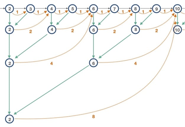
We can perform this merging step on each "level" of BLAs, creating 2-iteration BLAs from the 1-iteration ones, then creating 4-iteration BLAs from the 2-iteration ones, and so on, until we run out of BLAs to merge. At the end of this process, we'll have the single largest BLA, at the highest "level", for the first BLA iteration:

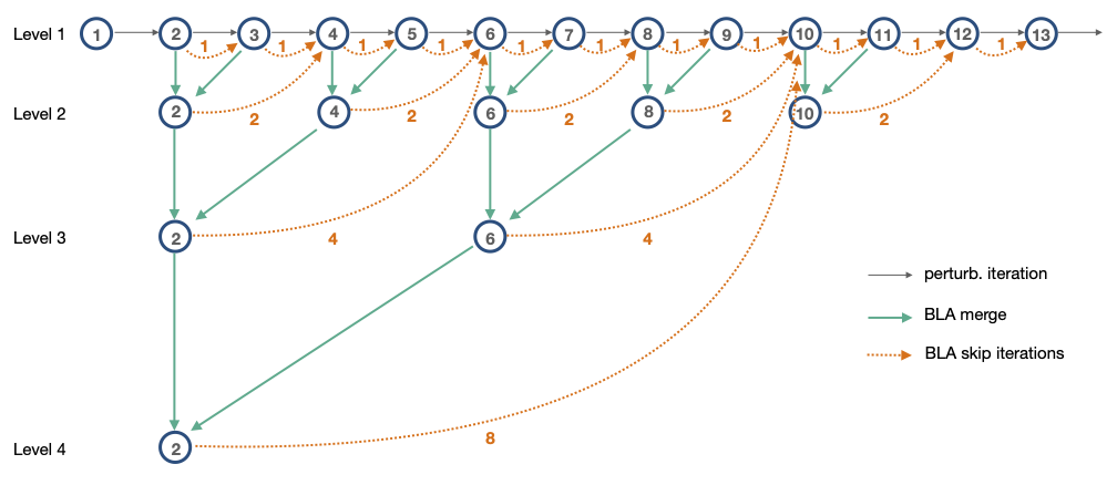
In the diagram above, each circle represents a Mandelbrot set iteration. The gray arrows represent regular perturbation theory iterations to move sequentially from one iteration to the next. The orange dotted arrows represent iterations that can be skipped by applying a BLA. For the "Level 1" BLAs, we "skip" only a single iteration. Adjacent pairs of "Level 1" BLAs are merged to create 2-iteration "Level 2" BLAs. We merge all the way to the largest BLA, at "Level 4" which can skip 8 iterations.

BLA Validity Checking

For each iteration we run, we have to efficiently test BLAs to find the largest valid one, or, if no valid BLAs are found, advance to the next iteration by running a regular perturbation theory iteration.

I tested a few algorithms for finding the best valid BLA at an iteration, and ended up using a simple linear search:

1. Test the lowest-level BLA
   • If valid, proceed
   • If not valid, end here: no BLAs at this iteration are valid
2. Test the highest-level BLA
   • If valid, stop: we have found the best BLA at this iteration
   • If not valid, repeat this step with the next-highest level BLA

Since the validity radius gets progressively smaller as we move from lower-level BLAs to higher-level BLAs, we know we can stop checking immediately if the lowest-level BLA is not valid. Then, since we want to apply the largest possible BLA, we can simply test the rest in descending order.

For example, in the diagram above:

At iteration 1, there are no BLAs, so apply a perturbation theory iteration to move to iteration 2.

At iteration 2, we first test the "Level 1" BLA. If valid, we then test the "Level 4" BLA. Say that's valid, and we can apply that BLA to end up at iteration 10.

Then at iteration 10, we continue this algorithm.

Note that as mentioned above, with the "merge and cull" strategy the BLAs at levels 1 and 2 are dropped in the actual implementation: it's not worth doing the BLA validity checking to advance only 1 or 2 iterations.

Epsilon

The key to the whole concept of BLA is the $\epsilon$ (epsilon) value. Recall that when the squared term in the perturbation equation value is "small enough" to be negligible we can apply the linear approximation to skip many iterations, where "small enough" means less than the non-squared term by some factor $\epsilon$:

$$\left|{\mathrm{\Delta }z}_n^2\right|<\epsilon \left|2Z_n{\mathrm{\Delta }z}_n\right|$$

In the fractalforums.org discussion on this, this $\epsilon$ value is directly based on the implementation to the underlying number values being used for the calculations. In this post, Zhuoran gives values of $\epsilon =2\times {10}^{-24}$ for single-precision floating-point values, and $\epsilon =2\times {10}^{-53}$ for double-precision.

I found those values to be fine in some of my initial testing, but noticed severe distortion or even totally wrong results being rendered in other cases. In general, it looks like smaller $\epsilon$ values must be used when "zooming" into a deeper locations, even when the math/number implementation doesn't change.

Auto-Epsilon

In my experimentation I found that for most locations, when the $\epsilon$ value is made a little smaller than it needs to be, the rendered images look accurate but fewer iterations are skipped with BLA (and thus take longer to render). Or, if the $\epsilon$ is made a little larger than optimal, the image can often look mostly the same (slightly inaccurate) and is rendered faster. Make it too large, however, and strange totally inaccurate results are rendered.

Using the above, I realized we can algorithmically find a good $\epsilon$ for any location:

1. Use regular perturbation theory to calculate the "true" iterations count value for a series of test points
2. Starting with some $\epsilon$ value, compute BLAs and compare the BLA-accelerated iterations result with the "true" perturbation result
3. If any point has a perturbation/BLA difference exceeding some threshold (I use 0.001%) then the $\epsilon$ is considered "wrong" and a smaller (more accurate, slower) $\epsilon$ value is needed
4. If all test points are correct, then compare the average number of iterations skipped vs the previous "best" $\epsilon$ value. If more iterations are skipped, then try a larger (less accurate, faster) value for $\epsilon$.

I implemented the above idea using a binary search, where the $\epsilon$ exponent is doubled or halved to find lower/upper bounds, and then the midpoint exponent is tested to repeatedly approach the "good" value. Since BLAs are relatively fast to calculate for each new $\epsilon$ value tested, we can quickly arrive at a $\epsilon$ value that produces fast, accurate results for the points tested.

Manual Epsilon

If a good $\epsilon$ is known for a particular location, or for testing a specific $\epsilon$ value, Very Plotter's "algorithm" parameter string can specify the value to be used (instead of using the "auto $\epsilon$" algorithm described above).

The algorithm string can be set in the "algorithm options" pane of the controls menu, or in the URL bar.

For example, to use $\epsilon =1\times {10}^{-114}$ at a scale that requires floatexp math, the algorithm can be specified as bla-floatexp-blaepsilon1.0eminus114.

To use $\epsilon =1.5\times {10}^{-26}$ at a scale that requires float math, the algorithm can be specified as bla-float-blaepsilon1.5eminus26.

Again, for all locations, the above auto-discovered $\epsilon$ value should work well, and BLA can be used by specifying the bla-auto algorithm.

Speed Comparison

To get a sense for BLA's performance, I've rendered a number of locations with both BLA and the previous fastest SA algorithm (perturbation theory with series approximation). Even with the additional initial computation steps (locating a minibrot nucleus, and calculating several sets of BLAs to find the best $\epsilon$) BLA is often much faster than SA.

All times below are for my M1 Mac, with 7 worker threads, rendering a relatively small 828x587 resolution window. I used a small window to speed up the test renders, but since BLA relies so much on the initial computation that occurs before any pixels are calculated, BLA should be even faster relative to SA for renders with many more pixels.

The images below are links that can be clicked to open the associated locations in Very Plotter. Some of the deeper locations take an extremely long time to render. Those slow locations are linked below more for future reference and performance measurement.

Example Location 1

This location is a deeper continuation from the "1" preset in Very Plotter. BLA shows an impressive speed improvement:

• 99s with BLA (about 1.5 minutes, with bla-float algorithm)
• 1009s (10.2x as long as BLA!) using perturb. theory with series approximation (with perturb-sapx6-float)

Example Location 2

This location is a deeper continuation from my "Cerebral Spin" location. It renders much more quickly with BLA:

• 358s with BLA (about 6 minutes, with bla-float algorithm)
• 12,958s (about 3.6 hours, 36.2x as long as BLA!!) using perturb. theory with series approximation (with perturb-sapx7-float)

Example Location 3

This is a location by Dinkydau, called "SSSSSSSSSSSSSSSS". This is where I first saw how the $\epsilon$ value may be dramatically different from one location to another. This location takes a long time to do the initial nucleus-finding and reference orbit steps, so I don't recommend actually viewing it with BLA! The SA render was somewhat faster than BLA, at least for the small test window. For a larger window, I hoped BLA would be faster.

• 3,438s with BLA (about 57 minutes, with bla-floatexp)
• 2,076s (about 35 minutes, 0.6x as long as BLA) using perturb. theory with series approximation (with perturb-sapx8-floatexp)

This is an interesting location because BLA appears to be slower, or not much faster, than SA. If and when I am able to make improvements to BLA, I'll be able to re-visit this location again to see if BLA gains any performance relative to SA.

I was hoping that, per pixel, BLA is slightly faster than SA here. If so, the initial nucleus-finding time would mean that only large renders would be faster with BLA. This was a mostly unnecessary tangent to follow, but I wanted to see if BLA appeared to be actually faster than SA, and, if so, whether I could predict the number of megapixels beyond which a BLA render would be faster overall than an SA render. I usually do 23-megapixel renders for gallery images (which I then downsample for a cleaner-looking 5.76-megapixel final image), so I'm also curious to see if BLA would be faster for a render of that size.

To test this, I guessed that I should be able to plot the time-vs-megapixels data as a best-fit line for both BLA and SA and see where the lines cross. Beyond that many pixels, BLA should be faster. To make a more accurate trend line, I ran renders for both BLA and SA. Since the $\epsilon$ for BLA can change depending on the render size and aspect ratio, I ran the following renders all at a 16:9 aspect ratio.

window	megapixels	BLA	SA	SA/BLA ratio
641x356	0.228	1,438s	1,045	0.727
928x522	0.486	2,608s	2,066s	0.792
1250x703	0.879	4,444s	3,595	0.809
1600x900	1.440	7,068s	5,805s	0.821
2311x1300	3.004	14,092s	11,917s	0.846

The auto-epsilon testing algorithm uses more test points for larger renders, so BLA's initial $\epsilon$-finding time also increases linearly with render size, but it shouldn't add much time overall. I was surprised to see that, even with the variable number of test points, the $\epsilon$ used was always $\epsilon =1\times {10}^{-122}$.

Plugging the BLA data into WolframAlpha gives a best fit line of:

$$y_{\text{seconds:BLA}}=4561.69x_{\text{megapixels}}+422.22$$

Which I interpret as 422 seconds (initial compute time for nucleus-finding, reference orbit, and BLA computation), plus 4561 seconds per megapixel.

And the SA data best-fit line of:

$$y_{\text{seconds:SA}}=3915.47x_{\text{megapixels}}+158.062$$

Which I interpret as 158 seconds (initial compute time for reference orbit and SA coefficients), plus 3915 seconds per megapixel.

Since the BLA equation starts with a higher initial compute time, and requires more seconds per megapixel, it will always be slower, at this location, than SA. I'll definitely re-visit this location in the future since it's a good benchmark for BLA vs. SA performance.

For this location I've also created an animation showing the effect of changing the value of $\epsilon$:

Example Location 4

This location is "Mandelbrot Deep Julia Morphing 31" by Microfractal on deviantart.com. This location takes an extremely long time to do the initial nucleus-finding and reference orbit steps, so again here I don't recommend actually viewing it in Very Plotter!

This location took such a long time to render (multiple days, where I often reduced the worker count down to 1 or 2 workers so I could continue to use the computer) that I don't have an SA performance comparison for it. This was a useful, very deep, location for testing BLA and the auto-epsilon algorithm.

A larger render of this location is available on the 2023 Mandelbrot set gallery page.

Example Location 5

This is the "Flake" location, by Dinkydau. A larger render of this location is available on the 2022 Mandelbrot set gallery page.

• 58s with BLA (bla-float algorithm)
• 89s (1.5x as long as BLA!) with perturb. theory with series approximation (perturb-sapx9.2-float)

For a larger 1600x900 window, with 6 workers:

• 220s with BLA (about 3.5 minutes, with bla-float)
• 536s (about 9 minutes, 2.4x as long as BLA!) with perturb. theory with series approximation (perturb-sapx9.2-float)

Example Location 6

This is the "Evolution of Trees" location, by Dinkydau.

• 3882s with BLA (about 64 minutes, with bla-float, skipping on average 989,000 iterations per pixel)
• 6553s (1.7x as long as BLA!) with perturb. theory with series approximation (perturb-sapx9-float, skipping 1,063,940 iterations per pixel)

Closing Thoughts

Implementing BLA was a serious challenge for me. It took several tries, but now Very Plotter is at the point where it's working well enough for the v0.10.0 release. This was a big undertaking, not just for BLA but for this 1100-line blog post as well!

It was very rewarding to read through the fractalforums.org discussion on BLA (starting at the top of page 3 here) and get it working myself. I owe a lot to those forum contributors for their general spirit of openness and for sharing their hard-earned knowledge on these topics.

It's worth mentioning that BLA is not yet compatible with stripe average coloring, which was recently added to Very Plotter. This doesn't seem to matter too much because BLA works at very deep locations where stripe average coloring (at least as I've implemented it so far) isn't worth using.

I'd like to experiment with other strategies for efficiently computing, storing, and testing BLAs. I feel like even more performance gains are possible with a bit more tinkering. I'd also like to look into WebAssembly for handling some of the arbitrary-precision and floatexp math in Very Plotter, which might dramatically improve Very Plotter's BLA performance.

But those are tasks for another day.